Pivot table is used to sort, count or give the average of the data stored in a spreadsheet, Pivot tables are also useful for converting rows to columns etc.
Here are the steps to create a pivot table.
Step 1: Start MS Excel Application
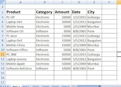
Step 2: Enter some data as following screen shot.
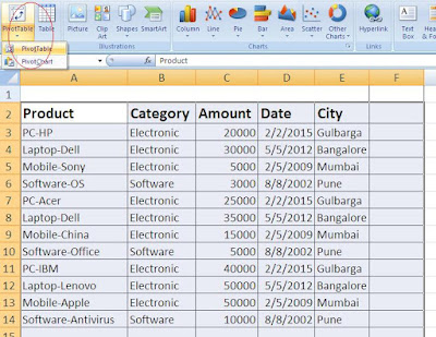
Step 3: Select your all data then click on “Insert” Tab and select “Pivot Table”, follow below image.
Step 4: Select “range of data or cells” with sheet, follow the below screen.

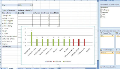
Step 5: Drag the fields as per following screen shot to summarize your all data.

Step 6: Chart can be created without much effort, just click on “chart” and it will opens different chart type and select “Column” type[for this example only] and the chart is ready!. [refer below screen shot]
Advantages of Pivot table:-
1) A pivot table will quickly summarizes the data by any column, calculate average, sum, count, percentage etc.
2) Data can presented in a chart.
3) Data can grouped by year, category wise or date etc.
