This example shows a simple marks calculation using MS-Excel.
Here are the steps for calculating total, average, minimum and maximum marks.
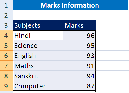
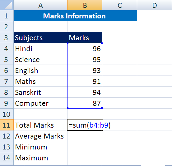
1. First of all, create a sheet with following data in it.
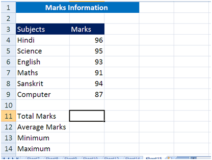
2. Place cursor next to “Total Marks” column and type the formula [while writing a formula in excel it is mandatory to put “=” equal sign before the formula or name of the expression and refer the cell address with separated by “:” colon, which indicates starting cell address and ending cell address] as shown in following image.
3. After hitting enter key you can see the following output.
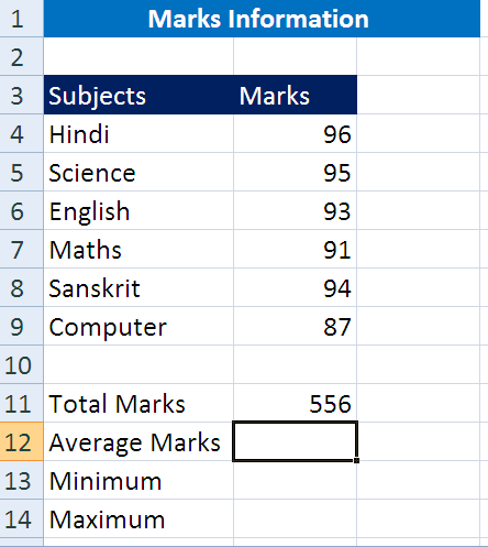
4. Now calculate Average. [follow below image]

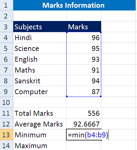
5. Now, find minimum value in the range. [follow below image]
6. Do also for Maximum. [refer below image]

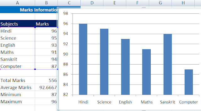
7. Now sheet looks completed with all 4 basic calculations- sum, average, minimum and maximum. [refer below screen shot]

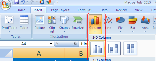
8. The above data can be shown in Graphical way .i.e. using excel “Charts”, just follow below steps.
8.a) First select all data as per following image.